Stream Processing
Overview
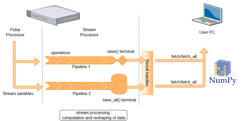
When saving data from a QUA program, it is first saved on the OPX on-board memory. From there, it's transferred to the server and eventually to the user PC. Stream processing provides the capability to process data as it is being transferred to the QM server. This both reduces the amount of data that has to be saved on the user PC, as well as the post-processing computation time.
Consider, as a simple example, a case where we would like to characterize the success rate of preparing a qubit in the \(|1 \rangle\) state. We want to play the pulse, read-out the qubit's state and decide whether it is a \(|1\rangle\) or a \(|0\rangle\). We then repeat this a large number of times, say \(1 \times 10^5\). Collecting the results of all \(10^5\) experiments is not so interesting. Instead, we can only collect the final average of the set of experiments or how this average develops as data is accumulated.
A running average is a straightforward example, but many other manipulations are possible. The "stream processing" allows for arithmetic operations and data reshaping to occur on server, in parallel to OPX experimental runs.
Basic Syntax and Examples
To use the server processing feature, a stream must be defined. A stream consists of a stream variable, a pipeline and a terminal. The processed stream items can be accessed on the client PC, where they are referred to as results, by creating result handles on the client PC. In what follows, we introduce each of these components and explain how they are used.
To initiate a stream, we use declare_stream() to declare a stream variable, using the following syntax inside a QUA program:
To pass a variable to a stream, we use the save() statement or the measure() statement.
This creates a data transfer path through which stream items are processed and then saved to either
a permanent or overriding storage (see Glossary for more details).
To illustrate how pipelines and terminals are created and used, we show below a full QUA program which saves data to a stream, manipulates it and stores the results to terminals. In addition, you can take a look at a few examples in our GitHub library
with program() as prog:
    my_stream1 = declare_stream(adc_trace=True)
    my_stream2 = declare_stream()
    a = declare(fixed)
    assign(a, 0.3)
    save(a, my_stream2)
    measure('my_pulse', 'qe', my_stream1)
    with stream_processing():
        my_stream1.input1().with_timestamps().save('adc_results')
        my_stream2.save_all('a_results')
Here two streams are created. The first, my_stream1, is used to stream raw ADC samples.
The second, my_stream2, is used to stream the value of the QUA variable a.
The pipelines and terminals are defined under the with stream_processing() context. Pipelines initiate with a
stream variable and terminate with a [save()][qm.qua._ResultStream.save] or [save_all()][qm.qua._ResultStream.save_all]
function, which acts as a terminal. In this example the pipelines are
simple: The first selects only the data from analog input1 and adds timestamps to it. The second is immediately terminated.
The terminal used for the pipeline initiated with my_stream1 is a save terminal.
This is a memory-less terminal that holds only the last value transferred - this can result in data loss if data
is not fetched quickly enough from the client PC. The terminal is given the tag 'adc_results', which can later
referenced using a result handle.
The terminal for my_stream2 is a save_all terminal which does store all the results (up to a memory
limitation, see Server PC storage and data limitations). The tag for this terminal is 'a_results'.
To access the results on the client PC side, we create a Result handle. This allows us to retrieve ("fetch") the stream items on the client PC side, or to perform other query or storage operations on it. To continue our example:
job = qm.execute(prog)
res = job.result_handles
my_stream_res = res.adc_results.fetch_all()['value']
This example collects all results which were contained in the stream using the
fetch_all() method.
Alternatively, we can only get the most recent result by calling the fetch() method.
Note that both these methods are called on a result handle. This structure and its usage are described below.
Note
It is still possible to use the syntax from previous versions for creating a stream that is only terminated
using save_all() ([legacy save][../#legacy-save]). The following examples are equivalent:
Warning
Saving values to the same stream from different OPXs is not supported.
Streaming Raw ADC Results
The following is a simple example of a program that acquires a single raw ADC trace:
with program() as prog:
    adc_stream = declare_stream(adc_trace=True)
    measure('my_pulse', 'qe', adc_stream)

    with stream_processing():
        adc_stream.input1().save('raw_adc')
By setting adc_trace=True we specify that data should be grouped into individual ADC
traces and not passed on a sample-by-sample manner, such that each trace will be of size (1, measurement_duration).
Next, to populate the stream with results, we specify the relevant stream in the measure statement. Finally, in the
stream_processing context, the pipeline specifies that we acquire data from analog input 1, and save it with the tag raw_adc
which we can later refer to in the client PC.
Note
Setting adc_trace=True is equivalent to writing stream.buffer(pulse_len + 2*smearing).
See details on buffer below and here on smearing
To record a raw ADC stream, it is required to play a digital marker that is associated with the measurement element. Only samples that arrive while the digital trigger is on will be recorded in the stream pipeline. This means it is possible to "gate" the raw ADC stream by using different
sequences of digital waveforms in the readout operation used for the measure() command.

Important
The digital waveform only affects the raw ADC streams. It does not change the data used when processing the measurement using integration, demodulation etc.
Results Handles
The stream items stored in the save/save all terminals on the server PC can be fetched to the client PC using the
results_handles property of the QmJob() object.
The fields of the result_handles property contain references to the stream terminals, and their names are the
same as the tags given to the terminals.
A handle to a specific terminal with tag "my_result", for example, is accessed with
my_result = job.results_handles.get("my_result").
A shorthand notation for this is my_result = job.results_handles.my_result.
We can query both the state of a single result handle or that of the collection of all results handles.
For example, one can query the processing state using the is_processing() method,
or the wait_for_all_values() method to suspend python execution until either a timeout has occurred or
saving has completed.
In case the handle references results from a save terminal, we can also wait for a specific number of results
to arrive using the wait_for_values() method.
The number of stream items referenced by a specific result handle can be obtained by calling count_so_far()
on that handle, or equivalently by calling len(my_result).
Saving results in numpy format to a local variable is done using the fetch and fetch_all
methods as specified below.
We can also save results to the file system by calling save_to_store().
fetch and fetch_all
To transfer the results from the server PC to the client PC, fetch() and fetch_all() commands are called on a result
handle, for example:
where my_stream is the tag result tag given to the save/save_all terminal.
fetch collects the most recent result in the stream and fetch_all collects all saved data.
In the case a save terminal is used, fetch all is equivalent to fetch.
It is also possible to collect only a portion of the collected data by passing fetch a slice object.
For example, say your result stream contains [0,1,2,3,4,5,6,7,8,9].
fetch(0) returns 0, fetch(4) returns 4 and fetch(slice(2,5) returns [2,3,4,5]. Any valid python slice object can be used.
Warning
When fetching the data while using pause() - resume() with a save() command there is no guarantee that the data you fetch at a given moment is the data point from the current iteration. There can be some delay from the moment the data is acquired until it is available for fetching.
Moreover, the streams are a-synchronous. For example, the availability of the result I[j] might be a few moments before Q[j]. If you fetch the data before the data is available at the Q stream, you will end up with a mixed data point I[j],Q[j-1].
That means that it is better to use the save_all() command and fetch the desired data.
Using Stream Operators
Data Restructuring with buffer()
The buffer method allows reshaping of the incoming stream items using the buffer() operator.
For example:
Will result in a stream of number pairs. And
Will result in a stream of 2 by 2 matrices. This is useful inside a doubly nested for loop as we can loop over a pair of independent variables and save the resulting dependent variable with the correct structure. We can then perform additional processing. For example, we can perform a running average over the resulting matrix in the following way:
This allows us to collect the resulting matrix and observe how the average evolved with the subsequent runs in real-time.
Buffer limitations
It is not possible to process more than 100e6 buffered variables at the same time. This is true for total number of variable streamed at the same time.
For example in the following snippet of code, the first line can be processed by itself, adding the second line will drive the system behind its limitations:
Note
streaming a buffered variable with time stamps is akin to streaming double the amount of variable. When using
with_timestamps(), each variable should be calculated as two variables when considering this limitation.
Combining streams using the zip operator
Streams can be zipped together into tuples of results using the zip() stream operator.
This is similar to creating a buffer but combines data from two separate streams rather than reshaping a single one.
In this case, the zipped resulting stream will have a shape dictated by the number of zipped tuples.
Each element of this tuple is a named field value_i where i is the named field number (the index of the zipped stream).
A_stream.zip(B_stream).save_all("zipped_tuple")
...
zipped = job.result_handles.zipped_tuple.fetch_all()
zipped has a shaped based on the number of items n. It has two named fields: value_0 and value_1.
Mapping operations over streams with the map function
The map function allows you to perform an operation on each element in a stream. It becomes especially useful when combined with the buffer function because then operations can be
performed on each filled buffer. For example, one can generate a buffer of size 3, and average over the samples in each triplet of numbers in the buffer. This is done as follows:
There are multiple FUNCTIONS that can be used in this way. For example, FUNCTIONS.dot_product(), FUNCTIONS.multiply_by(scalar_or_vector). Both these have
shortcut operators, so you can simply use .multiply_by as an operator in a stream pipeline. However, not all function have a shortcut, and it's useful to learn what the options are.
Some of these functions are: demod, boolean_to_int,`fft`,`tuple_convolution`, convolution,`tuple_multiply` but there are others. You can use Python's introspection to see what is available.
Average on axis
When working with two-dimensional buffers, one can specify over which axis to average. For example, in the following three-dimensional buffer, averaging is done on the first (zero-eth) axis with the following syntax:
A_stream.buffer(axis2_size).buffer(axis1_size).buffer(axis0_size).map(FUNCTIONS.average(0)).save_all(f"avg_axis0")
A list of axis can also be passed, in which case averaging is done on all passed axes. This matches behavior in numpy for example.
A_stream[i].buffer(axis2_size).buffer(axis1_size).buffer(axis0_size).map(FUNCTIONS.average([0, 1, 2])).save_all(f"avg_axis012")
Flat data structure option
The data structure returned by calling fetch_all is a numpy structured array. In simple cases, where buffering is not used, the shape of this array is exactly given by the number of saved items. If time stamps are also included, there is a single column of values and a second column with timestamps.
If, however the data is buffered or manipulated in some way, the number of items in the output array will be the number of filled (or partially filled) buffers. For example, consider the following buffered stream
If we had 300 items entering the steam, the shape of the output stream numpy array is: 6 (10*5*6 = 300). Each numpy array item has shape 10 X 6, but because the inner dimensions are "hidden" this is not indexable in the way you might expect.
To modify this behavior, an option to "flatten" the result array has been added. This is called by passing the following parameter to fetch_all:
In this case, the result shape will have the shape (6,5,10) and indexing can be performed as is usual in numpy array.
If the flat_struct flag is used on zipped streams, each named field will have a shape as described for a single stream.
Stream Processing Arithmetics
It is possible to use the server to perform arithmetic operations on a single stream or between different streams.
A complete list of the possible operations can be found in _ResultStream(). In general, an operation
can be performed between a stream to itself, two different streams or a stream and a scalar. The operation is done
element-wise, so both streams need to be buffered identically. In the case of an operation between a stream and a scalar,
the operations must be done before buffering the stream.
Note
It is possible to do multiplication between a buffered stream and a vector using the multiply_by() function.
The vector length must be identical to the stream buffer.
Some simple syntax examples:
(stream + 1).save("example")  # Adding 1 to each element in the stream
(stream_1 + stream_2).buffer(5).save("example")  # Adding element-wise stream1 to stream2 and buffering the result
(stream_1.buffer(5) + stream_2.buffer(5)).save("example")  # First buffering the streams and then adding them to each other
((stream1+1)*3+(stream2+1)/2).buffer(5).average().save_all("example")  # A combination of stream and scalar arithmetics
Notice that lines two and three in the above examples will results in identical outputs.
Warning
An operation between two streams that have different total length will only occur a number of times equal to the shortest stream
in their order within the pipeline, regardless of the location of the save() command in the QUA program.
For example if stream1 has n items, and stream2 has m items, where m < n. The result
of (stream1+stream2).save_all() would be an array of length m, with the values of the first m elements in stream1 added
element-wise to stream2.
Examples
A simple example that shows the utility of stream arithmetic is the ability to calculate the variance of a measured variable during the measurement. In the figure below, we see the results of generating a random integer between 0 and 9 repeatedly, and streaming two streams as written below:
stream.average().save_all("average")
((stream*stream).average()-(stream.average()*stream.average())).save_all("variance")
where the first line stream the running average (in blue in the figure), and the second line calculate the variance and stream the results (in orange in the figure).

Fig. 2: Running average stream (blue) and the variance stream(orange) of a randomly generated number on the OPX+. The horizontal lines mark the theoretical average (blue) and variance (orange).
In the following example, we see the use of the histogram. By using the Time Tagging, we get an array of time stamps indicating at which point in the measurement we counted a pulse (simulating a photon). By repeating the time tagging measurement, we can stream the results in a histogram telling us how many pulses we counted in each time bin.
times_st.histogram([[i, i + (resolution - 1)] for i in range(0, meas_len, resolution)]).save("times_hist")
The above code line shows how to use the histogram in the stream processing where meas_len is the measurement length,
and resolution is the required histogram bin size.

Fig. 3: A histogram of the number of counts as a function of measurement time. The time bin resolution is 20ns.
Legacy Save
Prior to saving into explicitly declared streams, QUA's save mechanism was directly to a tag : save(var,'tag') where 'tag' is a string identifier.
When using this legacy saving mechanism the output can be retrieved without change, as below:
This retrieves both values and timestamps. Alternatively, if only values (or only timestamps) are needed, we have introduced the following notation:
fetch_only_values= job.result_handles.get("A").fetch_all(flat_struct=True)
fetch_only_timestamps= job.result_handles.get("A_timestamps").fetch_all(flat_struct=True)
This provides only values (or only timestamps) and is slightly more performant than the previous option. In future versions flat_struct=True the default option.
Server PC storage and data limitations
A save_all terminal will store in the all of the stream items created during the execution
of a QUA program as results in the permanent memory of the server PC.
The permanent memory of the server PC is large but not unlimited, and therefore it is possible in some cases
to create more results than can be stored at the server PC.
The server PC permanent memory can store up to 100GB of result data without danger of data-loss.
Warning
If more than 100GB are stored in the permanent memory, the data may be erased after a short time to ensure the permanent storage is not overfilled. To ensure that job results are not erased, always make sure that no more than 100GB of data are generated by the QUA program without being fetched.
The results will not be immediately erased from the server once they are fetched.
To clear the permanent storage and ensure that all of the 100GB are available, use the
clear_all_job_results() method.
Data loss notification
When collecting results from a stream, the system can usually estimate how much data is expected to be received.
For example, if the measure command plays a pulse with a duration of 1000 samples, we expect to collect
an output of that length. In cases where the expected amount of data does not match the received amount,
an error message will appear when the res.my_stream.fetch_all() or .fetch() commands are called.
It can also be manually checked by calling
Video Tutorials
Stream processing - introduction
Stream processing - save and save_all
Stream processing - buffer
Stream processing - averaging
Stream processing - average within a buffer
Stream processing - buffer.average.buffer
Stream_processing - advance example (part 1)
Stream_processing - advanced example (part 2)
Glossary
Stream Variable
- A source (or start point) of a pipeline, receives values of QUA variables or raw input samples as input.
Save Terminal
- An overriding named sink or (end point) of a pipeline that creates a result. Each new stream item received at this terminal, will override the previous. The result is a single item, the last one received in a stream
Warning
Using a save terminal can result in data loss. It is to be used only in cases where data loss is acceptable, such as streaming plots.
Save All Terminal
- A named sink or end point of a pipeline that creates a result, which stores all the stream items in the pipeline. All stream items are appended to the result, complete history of the stream is preserved
Pipeline
- An ordered collection of operations that is performed on an input stream to return a processed version of the stream (output stream) In the context of stream processing, it is the collection of operations that can be performed starting from a stream variable and terminating in a "save terminal" or "save all terminal" node
Stream
- An ordered set of values that are being sent from a QUA program into a pipeline. A stream is set up when a QUA program is started and is torn down when it is finished.
Stream item
- A single discrete unit of data of a stream.
- Can be one of the following:
-
- ICP result
-
- Single input sample from the controller
-
- An input trace vector (single measure statement)
-
It is possible to augment the timestamp to each item using
withTimestamp
Result
- The last or accumulated stream items that are created by save or save_all terminals, respectively
Result Handle
- An object through which results can be fetched